Session 6
1
2
Types
R has different types of objects.
class(mtcars)## [1] "data.frame"class(c(1, 2, 3))## [1] "numeric"class(c("Hello", "Goodbye"))## [1] "character"3
Data Frames
- Data frames are special type of object composed of multiple objects.
glimpse(mpg)## Rows: 234## Columns: 11## $ manufacturer <chr> "audi", "audi", "audi", "audi", "audi", "audi", "audi", "…## $ model <chr> "a4", "a4", "a4", "a4", "a4", "a4", "a4", "a4 quattro", "…## $ displ <dbl> 1.8, 1.8, 2.0, 2.0, 2.8, 2.8, 3.1, 1.8, 1.8, 2.0, 2.0, 2.…## $ year <int> 1999, 1999, 2008, 2008, 1999, 1999, 2008, 1999, 1999, 200…## $ cyl <int> 4, 4, 4, 4, 6, 6, 6, 4, 4, 4, 4, 6, 6, 6, 6, 6, 6, 8, 8, …## $ trans <chr> "auto(l5)", "manual(m5)", "manual(m6)", "auto(av)", "auto…## $ drv <chr> "f", "f", "f", "f", "f", "f", "f", "4", "4", "4", "4", "4…## $ cty <int> 18, 21, 20, 21, 16, 18, 18, 18, 16, 20, 19, 15, 17, 17, 1…## $ hwy <int> 29, 29, 31, 30, 26, 26, 27, 26, 25, 28, 27, 25, 25, 25, 2…## $ fl <chr> "p", "p", "p", "p", "p", "p", "p", "p", "p", "p", "p", "p…## $ class <chr> "compact", "compact", "compact", "compact", "compact", "c…4
The Manufacturer column
mpg %>% count(manufacturer)## # A tibble: 15 × 2## manufacturer n## <chr> <int>## 1 audi 18## 2 chevrolet 19## 3 dodge 37## 4 ford 25## 5 honda 9## 6 hyundai 14## 7 jeep 8## 8 land rover 4## 9 lincoln 3## 10 mercury 4## 11 nissan 13## 12 pontiac 5## 13 subaru 14## 14 toyota 34## 15 volkswagen 275
A new type
- Factors are used to represent categorical variables
mpg_2 <- mpg %>% mutate(manufacturer=as.factor(manufacturer))glimpse(mpg_2)## Rows: 234## Columns: 11## $ manufacturer <fct> audi, audi, audi, audi, audi, audi, audi, audi, audi, aud…## $ model <chr> "a4", "a4", "a4", "a4", "a4", "a4", "a4", "a4 quattro", "…## $ displ <dbl> 1.8, 1.8, 2.0, 2.0, 2.8, 2.8, 3.1, 1.8, 1.8, 2.0, 2.0, 2.…## $ year <int> 1999, 1999, 2008, 2008, 1999, 1999, 2008, 1999, 1999, 200…## $ cyl <int> 4, 4, 4, 4, 6, 6, 6, 4, 4, 4, 4, 6, 6, 6, 6, 6, 6, 8, 8, …## $ trans <chr> "auto(l5)", "manual(m5)", "manual(m6)", "auto(av)", "auto…## $ drv <chr> "f", "f", "f", "f", "f", "f", "f", "4", "4", "4", "4", "4…## $ cty <int> 18, 21, 20, 21, 16, 18, 18, 18, 16, 20, 19, 15, 17, 17, 1…## $ hwy <int> 29, 29, 31, 30, 26, 26, 27, 26, 25, 28, 27, 25, 25, 25, 2…## $ fl <chr> "p", "p", "p", "p", "p", "p", "p", "p", "p", "p", "p", "p…## $ class <chr> "compact", "compact", "compact", "compact", "compact", "c…6
Class of the vector
class(mpg_2$manufacturer)## [1] "factor"7
Factors
- Behind the scenes, each category of a factor is assigned to a numeric value.
- The levels
levels(mpg_2$manufacturer)## [1] "audi" "chevrolet" "dodge" "ford" "honda" ## [6] "hyundai" "jeep" "land rover" "lincoln" "mercury" ## [11] "nissan" "pontiac" "subaru" "toyota" "volkswagen"- In this case, audi is 1, chevrolet 2, etc.
- The order of the levels is this codification.
- It is separate from the order in which the data frame is arranged.
8
Forcats
This package has functions to change the order of a factor. Think carefully about what you want.
fct_inorder(): by the order in which they first appear.In this case, the alphabetical order is the same as the order in which they appear in the data. This might not be true.
9
fct_infreq
fct_infreq(): by number of observations with each level (largest first)
mpg_3 <- mpg %>% mutate(manufacturer=fct_infreq(manufacturer))levels(mpg_3$manufacturer)## [1] "dodge" "toyota" "volkswagen" "ford" "chevrolet" ## [6] "audi" "hyundai" "subaru" "nissan" "honda" ## [11] "jeep" "pontiac" "land rover" "mercury" "lincoln"10
Example
- In the NBA data,
Team,Playoff,ConferenceandDivisionare factors.
nba <- readRDS('./nba.rds')glimpse(nba)## Rows: 30## Columns: 28## $ Team <chr> "Atlanta Hawks", "Boston Celtics", "Brooklyn Nets", "Charlo…## $ Playoff <fct> N, Y, N, N, N, Y, N, N, N, Y, Y, Y, N, N, N, Y, Y, Y, Y, N,…## $ GP <int> 82, 82, 82, 82, 82, 82, 82, 82, 82, 82, 82, 82, 82, 82, 82,…## $ MIN <int> 3941, 3961, 3971, 3956, 3971, 3946, 3961, 3976, 3961, 3946,…## $ PTS <int> 8475, 8529, 8741, 8874, 8440, 9091, 8390, 9020, 8509, 9304,…## $ W <int> 24, 55, 28, 36, 27, 50, 24, 46, 39, 58, 65, 48, 42, 35, 22,…## $ L <int> 58, 27, 54, 46, 55, 32, 58, 36, 43, 24, 17, 34, 40, 47, 60,…## $ P2M <int> 2213, 2202, 2095, 2373, 2264, 2330, 2161, 2398, 2322, 2583,…## $ P2A <int> 4471, 4483, 4190, 4873, 4736, 4314, 4354, 4566, 4756, 4611,…## $ P2p <dbl> 49.49676, 49.11889, 50.00000, 48.69690, 47.80405, 54.01020,…## $ P3M <int> 917, 939, 1041, 824, 906, 981, 967, 940, 886, 926, 1256, 74…## $ P3A <int> 2544, 2492, 2924, 2233, 2549, 2636, 2688, 2536, 2373, 2369,…## $ P3p <dbl> 36.04560, 37.68058, 35.60192, 36.90103, 35.54335, 37.21548,…## $ FTM <int> 1298, 1308, 1428, 1656, 1194, 1488, 1167, 1404, 1207, 1360,…## $ FTA <int> 1654, 1697, 1850, 2216, 1574, 1909, 1530, 1830, 1621, 1668,…## $ FTp <dbl> 78.47642, 77.07720, 77.18919, 74.72924, 75.85769, 77.94657,…## $ OREB <int> 743, 767, 792, 827, 790, 694, 666, 902, 830, 691, 739, 788,…## $ DREB <int> 2693, 2878, 2852, 2901, 2873, 2761, 2717, 2748, 2756, 2877,…## $ AST <int> 1946, 1842, 1941, 1770, 1923, 1916, 1858, 2059, 1868, 2402,…## $ TOV <int> 1276, 1149, 1245, 1041, 1147, 1126, 1007, 1227, 1103, 1265,…## $ STL <int> 638, 604, 512, 559, 626, 582, 578, 627, 628, 655, 699, 721,…## $ BLK <int> 348, 373, 390, 373, 289, 312, 310, 404, 317, 612, 392, 340,…## $ PF <int> 1606, 1618, 1688, 1409, 1571, 1524, 1578, 1533, 1508, 1607,…## $ PM <int> -447, 294, -307, 21, -577, 77, -249, 121, -12, 490, 695, 11…## $ team <fct> ATL, BOS, BKN, CHA, CHI, CLE, DAL, DEN, DET, GSW, HOU, IND,…## $ Conference <fct> E, E, E, E, E, E, W, W, E, W, W, E, W, W, W, E, E, W, W, E,…## $ Division <fct> Southeast, Atlantic, Atlantic, Southeast, Central, Central,…## $ Rank <int> 15, 2, 12, 10, 13, 4, 13, 9, 9, 2, 1, 5, 10, 11, 14, 6, 7, …11
Visualization
- Create a barchart of the number of 3 Pts attempts for the season. Add color to the bars to show if each team made the playoffs.
12
ggplot(data=nba, mapping=aes(Team, P3A)) + geom_col()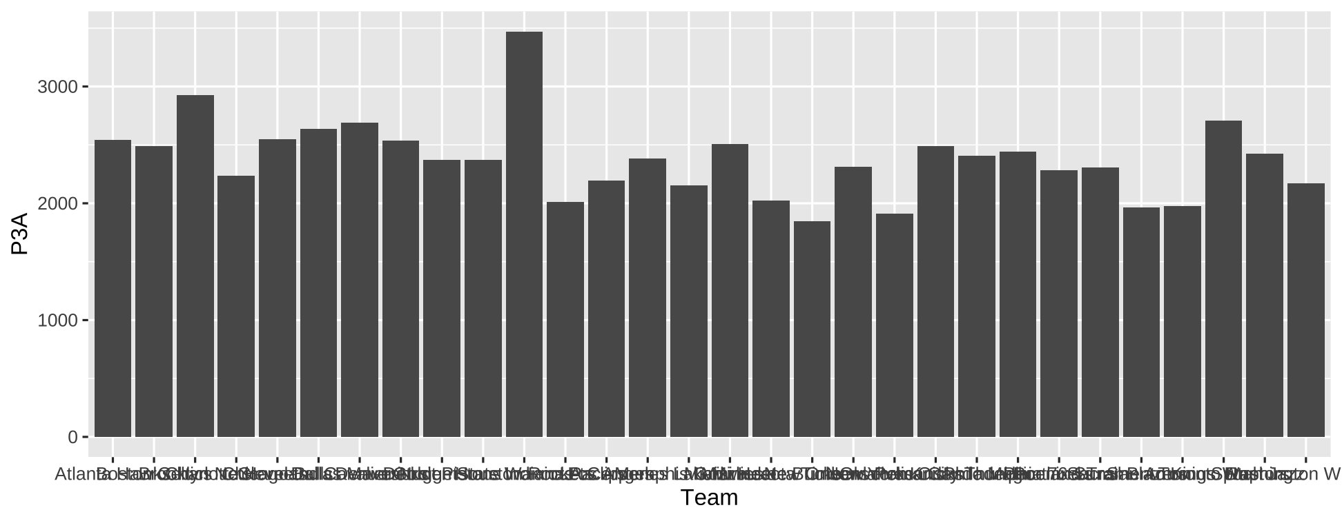
13
Example (2)
Flipping coordinates is useful to show the labels of the Teams.
ggplot(nba, aes(Team, P3A)) + geom_col() + coord_flip()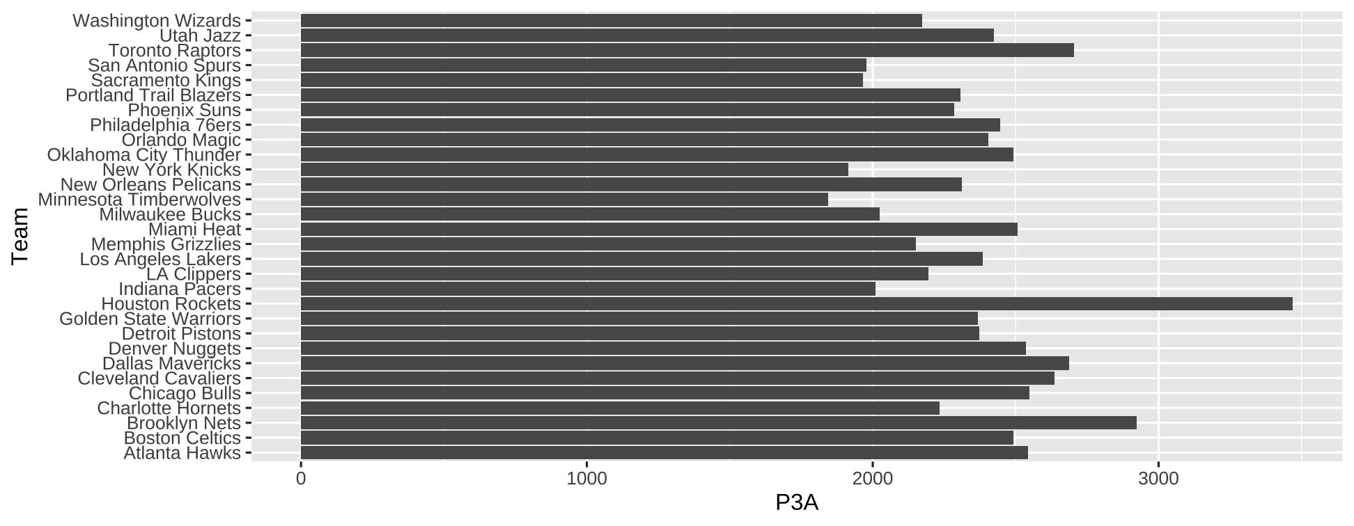
14
Order the factor
fct_reorderReorders the factor by another variable.
nba %>% mutate(Team=fct_reorder(Team, P3A)) %>% ggplot(aes(Team, P3A, fill=Playoff)) + geom_col() + coord_flip()
15
Function arguments and defaults
- You can pass arguments with or without names to functions
nba_data <- nba %>% mutate(Team=fct_reorder(Team, P3A)) ggplot(data=nba_data, mapping=aes(x=Team, y=P3A, fill=Playoff)) + geom_col() + coord_flip()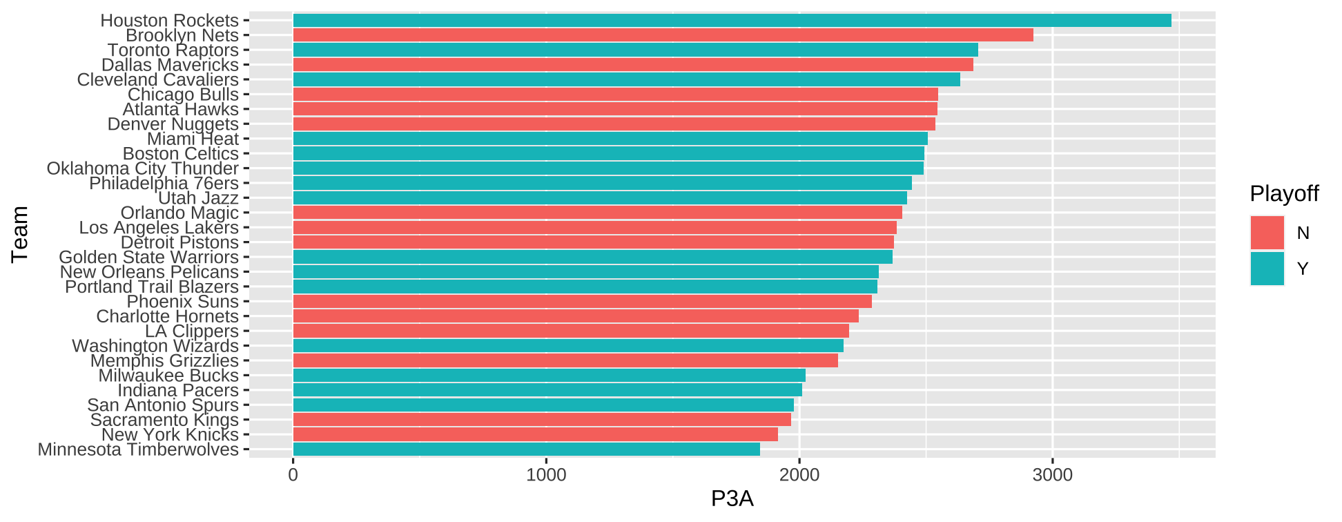
ggplot(nba, aes(P2A,P3A)) + geom_point()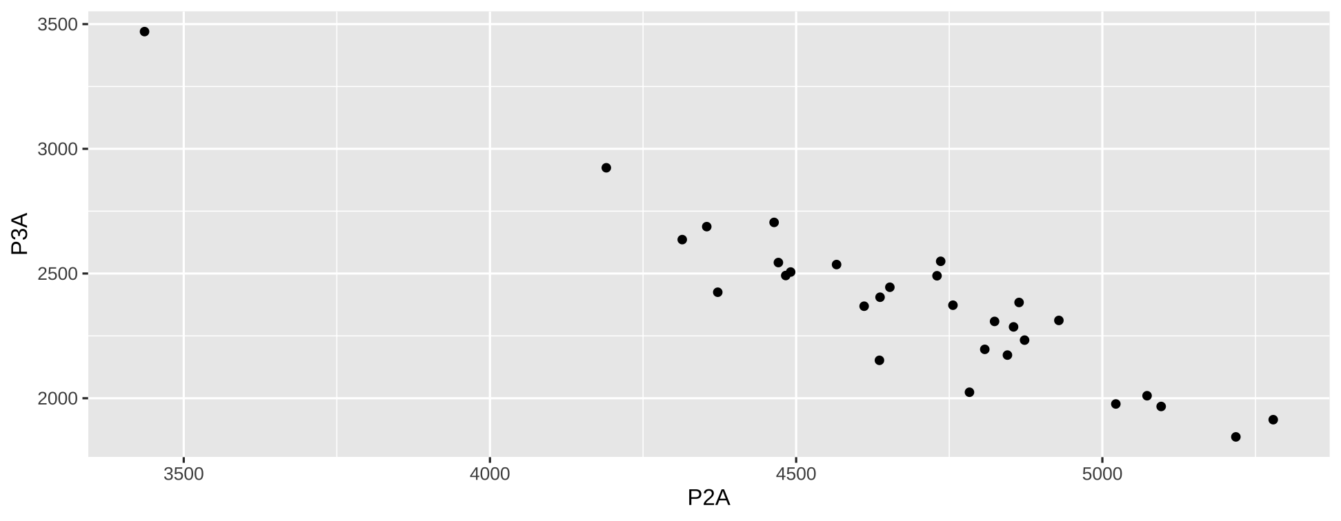
16
Time series plots
df <- read_excel('./mpd2018.xlsx', sheet = 'Full data')df_uy_usa <- df %>% filter(country %in% c("Uruguay", "United States"))plt <- df_uy_usa %>% filter(year>1800) %>% ggplot(aes(year, cgdppc)) + geom_line(aes(group=country, color=country)) + scale_color_discrete("") + labs(title="USA leaves Uruguay behind", subtitle="Income gap widened last century", x="Year", y="Per Capita GDP") + theme_minimal() + theme(legend.position = "bottom")17
plt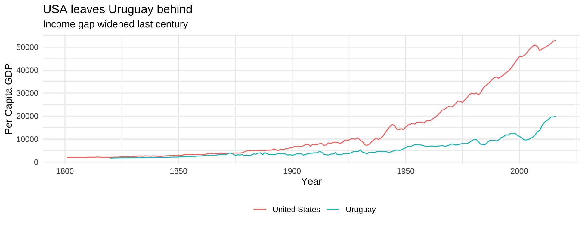
18
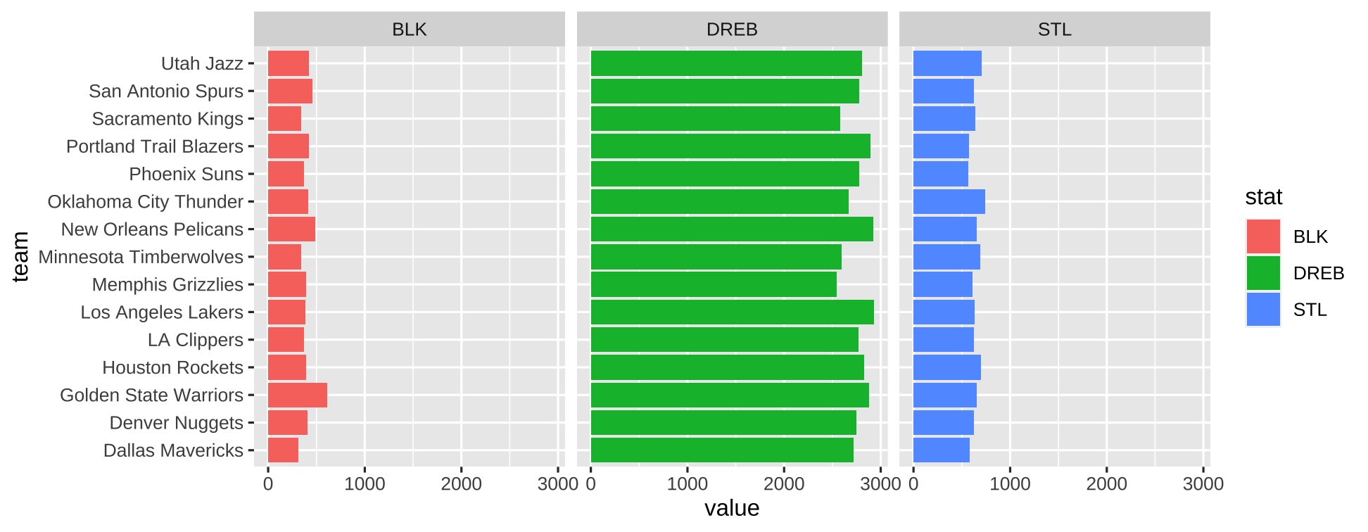
Facets
- Facets allow us to see different subsets of our data in different panes.
19
Facets in ggplot
- If we add a facetting layer to our ggplot, we get one pane for each subset of our facetting variable.
xw_long <- readRDS('./xw_long.rds')glimpse(xw_long)## Rows: 360## Columns: 4## $ team <chr> "Dallas Mavericks", "Dallas Mavericks", "Dallas Mavericks", "Dal…## $ conf <fct> W, W, W, W, W, W, W, W, W, W, W, W, W, W, W, W, W, W, W, W, W, W…## $ stat <chr> "GP", "MIN", "PTS", "W", "L", "P2M", "P2A", "P2p", "P3M", "P3A",…## $ value <dbl> 82.00000, 3961.00000, 8390.00000, 24.00000, 58.00000, 2161.00000…21
Facets
stats_plot <- xw_long %>% filter(stat %in% c("STL","BLK","DREB")) %>% ggplot(aes(x=team, y=value, fill=stat)) + geom_col() + coord_flip() + facet_grid(~stat)22
23
Scales
24